COTT Calculator
architecture guide
---
The COTT Calculator is a Python/SymPy implementation of Traction Theory's algebra,
with a tkinter calculator GUI, phase-plot visualizer, fractal engine,
and Chebyshev ring decomposition engine.
It lives under /solver
and comprises roughly 11,000 lines across two dozen files.
The solver is built on two core principles inherited from Traction Theory: totality (all operations defined for all values) and reversibility (no information loss). These principles drive every design decision — from zero having a reciprocal, to the universal power-of-power rule that eliminates branch cuts.
| File | Purpose |
|---|---|
traction.py |
Core algebra engine: types (Zero, Omega, Null, GradedElement), simplifier, projection, logarithms |
parser.py |
Recursive descent parser: expressions, equations, functions (solve, expand, factor, log0, logw) |
calculator.py |
Entry point and public API re-exports for backward compatibility |
evaluator.py |
Numeric traction evaluator: TractionValue class with zero/omega class tracking |
formatting.py |
Display formatting: exact, approximate, complex projection, and numeric modes |
decomposition.py |
Chebyshev ring decomposition engine: auto-detects band, reduces, evaluates |
visualization.py |
Phase grid computation and RGB mapping (phase mode and continuity mode) |
fractal.py |
Escape-time fractal engine with smooth HSV colouring |
streamlines.py |
Gradient streamline computation (tangent and normal flow lines via RK2) |
registry.py |
General-purpose function registry (category → name → object) |
chebyshev_ring.py |
Exact arithmetic: QsPoly, Element (a + b·u in ℚ[s][u]/(u²−su+1)),
TowerElement, MultiBandElement |
| projections/ | |
projections/base.py |
Base class for projection plugins |
projections/complex_lie.py |
Default projection: 0^z → e−Wz |
projections/geometric_algebra.py |
Geometric algebra: dot + wedge product, Cayley transform |
| gui/ | |
gui/app.py |
Main calculator window: five-tab UI, number pad, phase canvas, hover gauges |
gui/fullscreen.py |
Full-screen viewer with pan/zoom, progressive rendering, coordinate grid |
gui/settings.py |
Settings window: colour mode, projection selection, streamline toggles |
gui/constants.py |
Colour palette and layout constants |
gui/utils.py |
Tick formatting, colour scaling, line clipping utilities |
| Tests | |
test_traction.py |
160 pytest tests validating all traction identities |
test_chebyshev_ring.py |
173 tests for ring arithmetic, decomposition, and reduction |
traction.py)
Three custom SymPy Expr subclasses form the foundation.
They are not Symbols — they hook into SymPy's evaluation
via _eval_power, __mul__, and __truediv__.
| Class | Represents | Key behaviour |
|---|---|---|
Zero |
0 | Not absorbing. 0*w=1, 0^{-1}=w |
Omega |
ω | Reciprocal of zero. w*0=1, w^{-1}=0 |
Null |
∅ | Erasure element. Result of a-a=null |
Two additional classes handle unevaluated logarithms:
Log0 (base-0 logarithm)
and LogW (base-ω logarithm).
These are SymPy Function subclasses that stay symbolic
until projected to ℂ.
GradedElement (Zn) represents elements at grade n
in the operation hierarchy.
Grade arithmetic shifts operations one level:
Zn(a) + Zn(b)
= Zn−1(a·b),
and Zn(a) × Zn(b)
= Zn+1(a+b).
Fixed points: Zn(0) = Zn−1(1),
Zn(ω) = Zn−1(−1).
Z0 is the identity grade.
The parser accepts both Z_n(expr) and Z(n, expr) syntax.
_eval_power)
The _eval_power hooks fire during SymPy's Pow construction,
so most identities are enforced eagerly — no simplifier call needed:
| Identity | Generalised form |
|---|---|
| 0^0 = 1 | |
| 0^{-r} = w^r | Negative integer or rational exponent |
| 0^w = -1 | |
| 0^{0^n} = n | 0^{0^x} = x for any x |
| 0^{w^n} = -n | 0^{w^x} = -x for any x |
The generalisation beyond integers enables the resolve() identity-resolution
technique: wrapping any expression in 0^{0^{x}}
is a guaranteed no-op.
traction_simplify)
The simplifier is a recursive, bottom-up rewriter. It handles three expression types beyond the eager power rules:
Pow: Universal power-of-power: (v^a)^b = v^{a*b} for any base v, not just 0 and ω. This is what eliminates branch cuts — (x^2)^{1/2} = x, not |x|.
Mul:
All Zero and Omega factors are unified into a single base-0 exponent
using ωa = 0−a.
Exponents are summed:
0^a * 0^b = 0^{a+b},
0^a * w^b = 0^{a-b}.
After cancellation, the result is reconverted
(negative rational exponent → ω-base).
Signs are preserved:
-0 is a valid distinct expression
equal to ω in the reduced Chebyshev ring (see §6.3).
Add:
If the result is SymPy's S.Zero (from cancellation),
it is replaced with Null (the erasure element).
project_complex)
Projection maps traction expressions to ℂ. It is intentionally the last step in the pipeline — all traction simplification happens first, so branch cuts from classical complex arithmetic are avoided.
The core mapping is the Lie group exponential:
The structure constant W = √(−iπ) ≈ 1.253 − 1.253i, with |W| = √π. This single formula handles all base-0 powers:
| Traction | Projected | Verification |
|---|---|---|
| 0^0 | e0 = 1 | |
| 0^w | e−W² = eiπ = −1 | Consistent with 0^w = -1 |
| 0^{w/2} | eiπ/2 = i | The dyadic imaginary unit |
| 0^n (positive n) | e−nW, magnitude < 1 | Zero-class: decaying magnitude |
| 0^{-n} | enW, magnitude > 1 | Omega-class: growing magnitude |
A critical identity for projection: ω = W in exponent space. This is derived from the consistency equation:
This means: wherever ω appears inside an exponent or logarithm argument,
the projector substitutes ω → W before evaluating.
Without this, ω would project to ∞ (its standalone value),
producing zoo contamination.
Inverting the Lie exponential gives the logarithm projections:
The same ω → W substitution is applied to arguments
containing ω before the ln is evaluated.
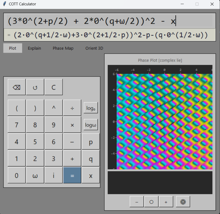
The visualizer renders phase plots (domain colouring) of traction expressions over a 2D grid. The pipeline is designed to stay in the traction domain as long as possible, projecting to ℂ only at the final step.
Expressions use three variables with distinct roles:
| Variable | Role | Substitution |
|---|---|---|
| p | Horizontal grid coordinate | Always the real horizontal axis |
| q | Vertical grid coordinate | Always the real vertical axis |
| x | Projection's native unit | Defined per projection (see below) |
| t | Time parameter | Scalar, controlled by slider in the GUI |
| c | Fractal parameter | Complex constant for escape-time iteration (the Mandelbrot c) |
p and q are projection-agnostic — they always map directly to the grid axes. x is the projection's native coordinate, meaning the same expression 0^x has different geometric meaning depending on which projection is active:
| Projection | x = | Interpretation |
|---|---|---|
| Complex Lie | p + q·0^{w/2} | Complex plane |
| Q-surface | 0^{p + q*0^{w/2}} | Complex plane lifted into zero-power domain |
All three variables may appear in the same expression: p^2 + x uses both raw coordinates and the native unit.
Step 1 — Parse:
Recursive descent parser converts the input string to a SymPy expression
with traction types (Zero, Omega, etc.).
Step 2 — Substitute:
Replace p → a,
q → b (real grid symbols),
and x → the active projection's native_x(a, b).
This substitution happens in the traction domain —
the expressions are still traction objects, not complex numbers.
Step 3 — Traction Simplify: Apply all traction rewrite rules. The universal power-of-power rule fires here, collapsing expressions like (x^2)^{1/2} → x before any complex arithmetic occurs. This is what eliminates branch cuts.
Step 4 — Project: The active projection converts the simplified traction expression to a form suitable for numeric evaluation. For Complex Lie, this applies 0^z → e−Wz. For Q-surface, it decomposes zero-powers into phase and magnitude coordinates.
Step 5 — Evaluate:
The projected expression is converted to a numpy vectorised function via
SymPy's lambdify and evaluated over the grid in one pass.
For scalar display (the result line), the TractionValue evaluator
(evaluator.py) provides class-tracked arithmetic:
a numeric type that tracks whether a value is a plain scalar, a zero-power
(0^{a+b*w}), or an omega-scaled quantity (result of division by zero).
Each arithmetic operation preserves the class distinction:
| Operation | Class transition |
|---|---|
| p / 0 | SCALAR → OMEGA_VAL(p) |
| 0 ^ OMEGA_VAL(p) | → ZERO_POWER with ω-exponent → eiπp |
| ZERO_POWER × ZERO_POWER | Exponents add: 0^a * 0^b = 0^{a+b} |
| Scalar near 0 in base | Promoted to traction 0 |
Long-running computations (fractal iteration, full-screen progressive render) run in a background thread, keeping the GUI responsive. Starting a new computation automatically cancels any in-progress one.
Step 6 — Colour: Two modes: Phase mode (CMYT quadrant colours, brightness by log-magnitude) and Continuity mode (CMYT following magnitude via double-cover arctan, ensuring |f|→0 and |f|→∞ have the same colour).
The key architectural decision: substitution and simplification happen in the traction domain, before any projection to ℂ. An earlier design projected first, then substituted:
expr → project → subs x→a+bi → numpy (branch cuts!)
This inherited all of ℂ's branch cut baggage. Fractional powers like (x^2)^{1/2} would hit numpy's principal-value convention, causing discontinuities on the imaginary axis. The native pipeline reverses the order:
expr → subs p,q,x → traction_simplify → project → evaluate
By the time the expression reaches numeric evaluation,
the traction simplifier has already collapsed the nested powers.
The branch cut never forms. And the TractionValue evaluator
preserves traction semantics at the numeric layer —
division by zero produces ω, not NaN.
Projections are modular. Each projection lives in its own
.py file under projections/
and self-registers into the global registry on import.
registry.py)
A general-purpose {category, name} → object store.
Not limited to projections — any subsystem can register functions,
strategies, or configuration under its own category.
Create a file in projections/ that subclasses Projection
from projections/base.py. Implement two methods:
project_expr(traction_expr, a, b) —
Convert a traction expression (containing symbols a,
b) to a form suitable for lambdify.
Handles variable detection and substitution mode (single-variable vs two-variable).
eval_grid(projected_expr, a, b, AA, BB) —
Lambdify, evaluate on the numpy meshgrid, and return a dictionary of 2D arrays:
{Z, Re, Im, mag, log_mag, phase, brightness}.
Call self.register_self() at module level. The
projections/__init__.py auto-imports all .py files
in the directory, triggering registration.
projections/geometric_algebra.py)
A purely algebraic alternative to the Lie exponential, grounded in 2D geometric algebra. The geometric product of two vectors decomposes as:
In 2D with basis vectors e1, e2, the bivector I = e1e2 is the oriented unit area element. Its square determines the algebra's character:
| Metric | I² | Exponential | Behavior |
|---|---|---|---|
| Circular (Lie) | −1 | cos θ + I sin θ | Rotation (phase) |
| Hyperbolic (GA) | +1 | cosh φ + I sinh φ | Boost (magnitude) |
Same algebraic structure, different metric signature → completely different behavior. A complex number a + bi becomes a multivector a + bI: the real part is a scalar, the imaginary part is an oriented area element.
Coloring derives from the geometric product of input p and output f(p):
| Product | Formula | Meaning |
|---|---|---|
| Dot (scalar) | p·f(p) = xu + yv | Radial stretch / alignment |
| Wedge (bivector) | p∧f(p) = xv − yu | Oriented rotation / angular twist |
For zero-powers, the Cayley rational transform replaces the transcendental exponential: 0^z → (1+z)/(1−z) — conformal, rational, and unit-circle preserving. No exp, log, sin, cos, or atan2.
Zero and Omega are Expr subclasses
with _eval_power hooks. This means SymPy evaluates
0^w → −1 during construction
of the Pow object — no explicit simplify call needed.
Using plain Symbols would require a post-hoc rewriter for every expression.
In multiplication, all Zero and Omega factors
are converted to base-0 exponents
(ωa = 0−a),
summed, and reconverted. This single mechanism handles:
0*w=1 (exponents cancel),
0^2*w=0 (partial cancel),
0^a * 0^b = 0^{a+b} (symbolic combine),
and cross-base products like 0^5 * w^2 = 0^3.
-0 is a valid, distinct expression — the additive inverse of traction zero. In the Chebyshev ring, the identity 0 + w = null (additive inverse) combined with 0 * w = 1 (multiplicative inverse) forces ω = −0: since 0² = −1, we get ω = 0−1 = 0/0² = 0/(−1) = −0.
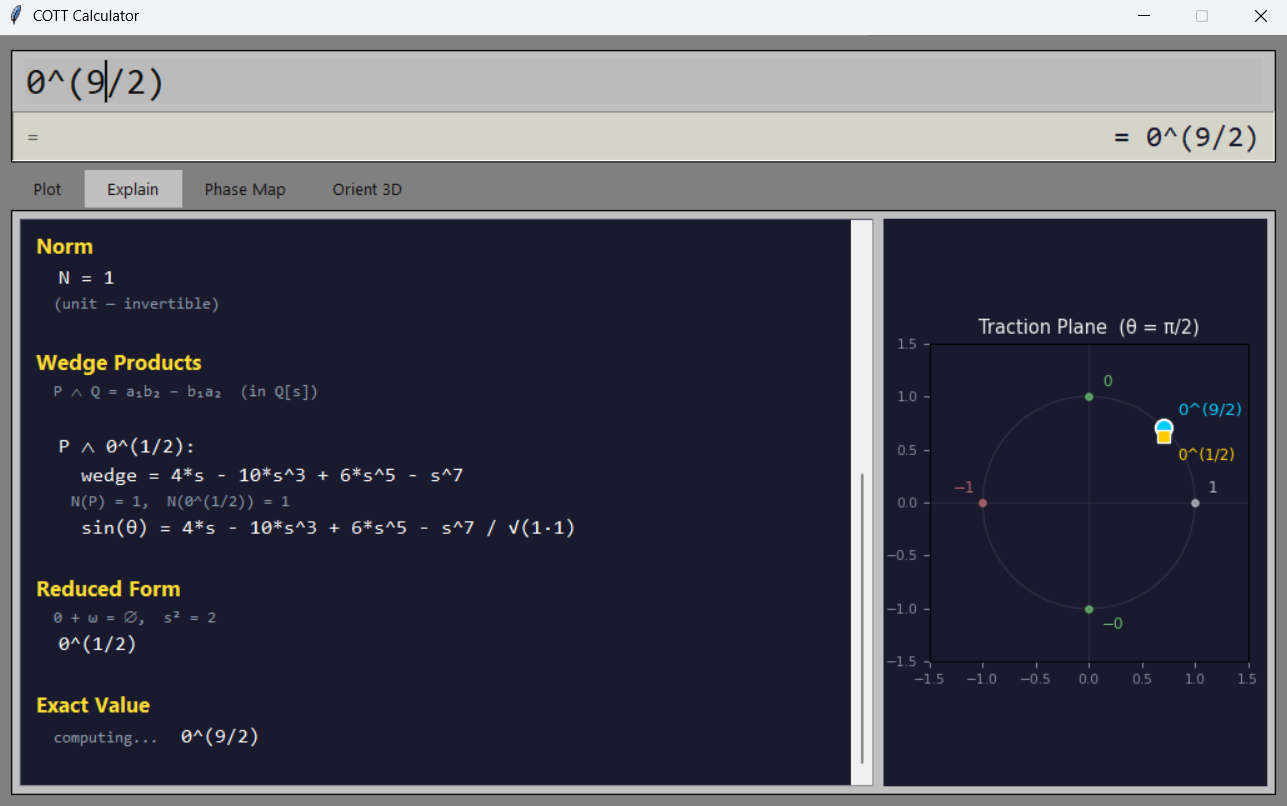
This single identity recovers the 8th roots of unity purely algebraically. The Explain tab's Reduced Form section computes this by reducing the ring polynomial modulo Tn(s/2) = 0 (the Chebyshev polynomial relation from 0 + ω = ∅) and substituting back:
| Expression | Reduced Form | Complex value (θ = π/2) |
|---|---|---|
| 0^0 | 1 | 1 |
| 0 | 0 | i |
| 0^2 | −1 | −1 |
| 0^3 | −0 | −i |
| 0^4 | 1 | 1 |
The Traction Plane plot displays these values with cardinal points 1 (right), −1 (left), 0 (top), −0 (bottom), confirming that traction zero acts as the imaginary unit i.
sp_simplify
SymPy's simplify() is deliberately avoided in the projection pipeline.
It aggressively rewrites expressions in ways that break numeric evaluation —
for instance, merging i·√r into √(−r),
which produces NaN for positive r.
Projected expressions are left in their natural factored form.
parser.py)
The parser is a hand-written recursive descent parser supporting
full operator precedence (parentheses, exponentiation, multiplication/division,
addition/subtraction) with right-associative ^.
| Syntax | Meaning |
|---|---|
log0(expr) |
Base-0 logarithm (symbolic until projected) |
logw(expr) |
Base-ω logarithm |
solve(expr) or solve(expr, var) |
Solve expr = 0 for var. Returns a SolutionSet. |
expand(expr) |
Symbolic expansion (distributes products over sums) |
factor(expr) |
Symbolic factoring |
The parser supports equation syntax: lhs = rhs is automatically
converted to solve(lhs − rhs) and solved.
The result is a single solution or a SolutionSet.
Graded elements can be entered as Z_n(expr) or Z(n, expr),
where n is the grade level.
These are first-class values: they can be combined with arithmetic operators,
and the grade algebra rules (see §2) apply automatically.
gui/)
The calculator GUI (gui/app.py) is a tkinter window with
an input display, a result display (with an ≈ toggle for approximation mode),
and a five-tab workspace:
| Tab | Contents |
|---|---|
| Plot | Calculator number pad (left) + phase-plot canvas with hover gauges, zoom controls, and settings (right) |
| Explain | Chebyshev ring decomposition text + orbit plot (matplotlib) |
| Phase Map | Interactive phase-amplitude decomposition at varying θ, with orbit, amplitude, and table subplots |
| Orient 3D | 3D tower visualisation with two rotation sliders (θw and θu) |
| Help | Scrollable, clickable examples organised by section |
The result display has an = / ≈ toggle button.
In exact mode, results display as symbolic traction expressions (fractions, Zn, etc.).
In approximation mode, rationals and complex values are displayed as decimals.
gui/fullscreen.py)
A dedicated full-screen window with pan and zoom. Uses dual-layer image buffers: a low-resolution persistent layer for instant feedback during interaction, and a high-resolution progressive layer rendered after a 200 ms debounce. Includes a coordinate grid overlay and legend.
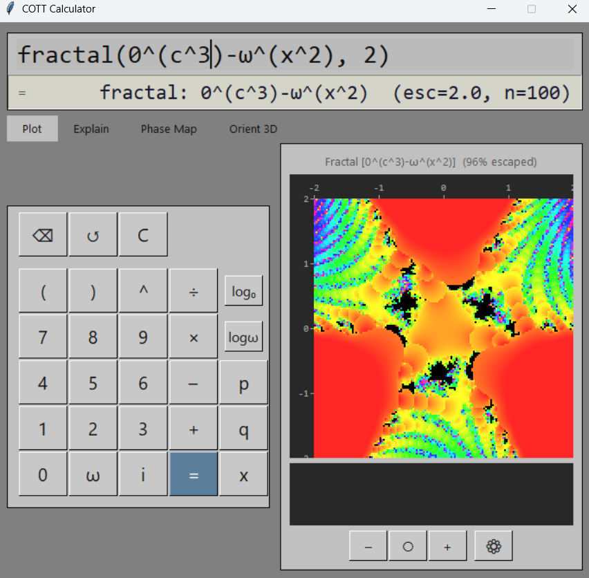
fractal.py)
Expressions containing the variable c trigger fractal (escape-time iteration) mode. The iterator starts at traction zero (x0 = 0, which projects to eiπ/2 = i under θ = π/2) and iterates the expression at each grid point. Colouring uses smooth HSV with anti-banding based on escape count and final magnitude.
gui/settings.py)
The settings window provides controls for: colour mode (phase or continuity), active projection (Complex Lie or Q-Surface), and gradient overlays (tangent lines following |f| gradient, normal lines following constant-|f| contours).
SymPy eager evaluation:
0^1 is eagerly simplified to Zero()
by _eval_power, losing the exponent information.
This means Pow(Zero(), 1) and bare Zero() are
indistinguishable to the projector — both project via
e−W.
Non-analytic two-variable mode: When p and q are used as independent real variables, the function is generally not analytic in the complex sense. Phase and magnitude gradients are independent, so the tangent/normal lines (which follow magnitude) may not align with the phase colouring. This is correct behaviour, not a bug.
Projection completeness: The Lie exponential projection is one of potentially many valid mappings from traction to ℂ. The plugin system exists specifically to allow alternative projections (e.g. rational-magnitude formulas) to be developed and compared.